Tutorial #3: Primitivization and Paths¶

Aims:

Build a primitive cell from the Atoms and InteractionList objects
Determine a suitable path in reciprocal space over which to plot a bandstructure

In the previous tutorial, we introduced a body-centred cubic cell. This cell contains two atoms, but it is not the primitive cell. This means that the two atoms are, in fact, copies of each other, which will lead to spurious additional bands. Therefore, we build a monatomic primitive cell from the provided diatomic conventional cell.

Initialize¶

As usual, we import the necessary modules:

import magnon
from ase import Atoms
import numpy as np

Structure and Coupling¶

Define the BCC iron structure. We use the magnetic moment of iron which is \(2.2\mu_B\):

lattice = np.array([[1, 0, 0],
                    [0, 1, 0],
                    [0, 0, 1]])
positions = np.array([[0, 0, 0], [0.5, 0.5, 0.5]])
magnetic_moments = np.array([[0.0, 0.0, 2.2], [0.0, 0.0, 2.2]])

atoms = Atoms(["Fe", "Fe"], positions=positions, cell=lattice)
atoms.set_initial_magnetic_moments(magnetic_moments)

Then define a minimal set of interactions up to second nearest-neighbour:

interactions = magnon.InteractionList([], atoms=atoms)
interactions.insert_interaction(0, 1, np.array([0.5, 0.5, 0.5]), 0.021*np.eye(3))
interactions.insert_interaction(0, 0, np.array([1.0, 0.0, 0.0]), 0.013*np.eye(3))
interactions.insert_interaction(1, 1, np.array([1.0, 0.0, 0.0]), 0.013*np.eye(3))

And symmetrize:

interactions = interactions.symmetrize(atoms)

Primitivization¶

The Atoms and InteractionList objects of the primitive cell are obtained using

atoms, interactions, _ = magnon.build.build_primitive_cell(atoms, interactions)

Note

It is good practice to symmetrize the exchange interaction before primitivizing. The reverse could result in missing couplings.

Paths in Reciprocal Space¶

To analyze the magnon bandstructure of complex materials, we wish to select a high-symmetry path through the Brillouin zone that reflects the material’s underlying crystal symmetry. SeeK-path is an open-source tool that automates this process using symmetry analysis based on the material’s structure. It can be used as a Python API or via the online interface. We create a POSCAR file:

IronBCC
1
        1.0000000000         0.0000000000         0.0000000000
        0.0000000000         1.0000000000         0.0000000000
        0.0000000000         0.0000000000         1.0000000000
   Fe
    2
Direct
     0.000000000         0.000000000         0.000000000
     0.500000000         0.500000000         0.500000000

and upload it to SeeK-Path. The recommended path is returned:

\[\Gamma—H—N—\Gamma—P—H\]

which can be supplied to an ASE bandpath with the Atoms object to generate the path:

path = atoms.get_cell().bandpath(path='GHNGPH', npoints=60)

We can finally initialize the MagnonSpectrum object with the structure and interactions, and plot the bandstructure:

spectrum = magnon.MagnonSpectrum(atoms, interactions)

bstruct = spectrum.get_band_structure(path)
bstruct.plot(emin=0, emax=0.7, filename='Iron_BCC_bands.png')

Full script¶

The combined script for all of the above is

import magnon
from ase import Atoms
import numpy as np

lattice = np.array([[1, 0, 0],
                    [0, 1, 0],
                    [0, 0, 1]])
positions = np.array([[0, 0, 0], [0.5, 0.5, 0.5]])
magnetic_moments = np.array([[0.0, 0.0, 2.2], [0.0, 0.0, 2.2]])

atoms = Atoms(["Fe", "Fe"], positions=positions, cell=lattice)
atoms.set_initial_magnetic_moments(magnetic_moments)

interactions = magnon.InteractionList([], atoms=atoms)
interactions.insert_interaction(0, 1, np.array([0.5, 0.5, 0.5]), 0.021*np.eye(3))
interactions.insert_interaction(0, 0, np.array([1.0, 0.0, 0.0]), 0.013*np.eye(3))
interactions.insert_interaction(1, 1, np.array([1.0, 0.0, 0.0]), 0.013*np.eye(3))

interactions = interactions.symmetrize(atoms)
atoms, interactions, _ = magnon.build.build_primitive_cell(atoms, interactions)

path = atoms.get_cell().bandpath(path='GHNGPH', npoints=60)

spectrum = magnon.MagnonSpectrum(atoms, interactions)

bstruct = spectrum.get_band_structure(path)
bstruct.plot(emin=0, emax=0.7, filename='Iron_BCC_bands.png')

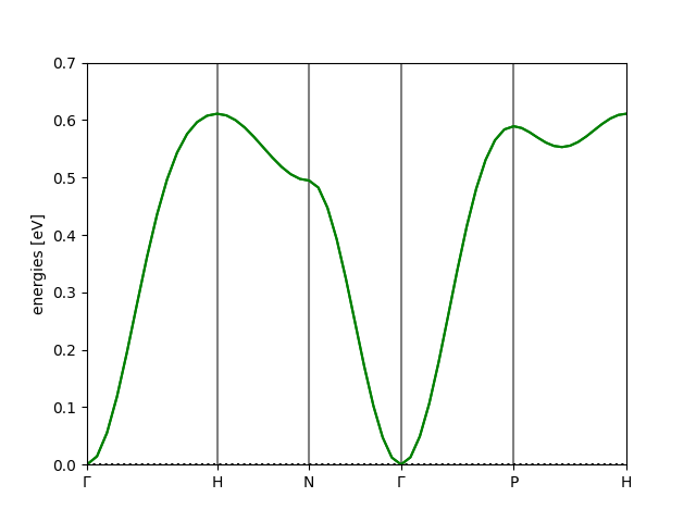
Result¶

The following figure shows the resulting Iron BCC magnon bandstructure:

Iron BCC magnon band structure in the primitive cell along a high-symmetry path

Spurious Folded Bands¶

Now consider what we would have obtained without the primitivization step. Consider the full script:

import magnon
from ase import Atoms
import numpy as np

lattice = np.array([[1, 0, 0],
                    [0, 1, 0],
                    [0, 0, 1]])
positions = np.array([[0, 0, 0], [0.5, 0.5, 0.5]])
magnetic_moments = np.array([[0.0, 0.0, 2.2], [0.0, 0.0, 2.2]])

atoms = Atoms(["Fe", "Fe"], positions=positions, cell=lattice)
atoms.set_initial_magnetic_moments(magnetic_moments)

interactions = magnon.InteractionList([], atoms=atoms)
interactions.insert_interaction(0, 1, np.array([0.5, 0.5, 0.5]), 0.021*np.eye(3))
interactions.insert_interaction(0, 0, np.array([1.0, 0.0, 0.0]), 0.013*np.eye(3))
interactions.insert_interaction(1, 1, np.array([1.0, 0.0, 0.0]), 0.013*np.eye(3))

interactions = interactions.symmetrize(atoms)
prim_atoms, prim_interactions, _ = magnon.build.build_primitive_cell(atoms, interactions)

path = prim_atoms.get_cell().bandpath(path='GHNGPH', npoints=180)

spectrum = magnon.MagnonSpectrum(atoms, interactions)

bstruct = spectrum.get_band_structure(path)
bstruct.plot(emin=0, emax=0.7, filename='Iron_BCC_bands_folded.png')

We keep the primitivization, but only use it to calculate the reciprocal space path - this ensures we are consistent with the horizontal axis of the plot. For the magnon bandstructure, we used the conventional two-atom cell. This results in the bands:

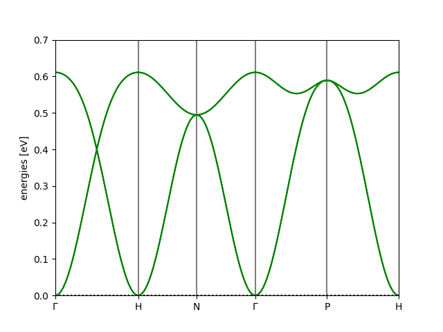
Iron BCC magnon band structure in the conventional cell along a high-symmetry path

This is the same as the first bandstructure plot, only the bands are ‘folded over’ to give a second, spurious copy. This is misleading, and shows the importance of using a minimal cell; it is flawed to treat periodic images as distinct atoms.